Chapter 01: Finite Sample Properties of OLS
Lachlan Deer
2019-03-04
Source:vignettes/chapter-01.Rmd
chapter-01.RmdApplication: Returns to Scale in Electricity Supply
Load the hayashir package
library(hayashir)The Data
Let’s get a quick look at our data by looking at the first 10 rows:
head(nerlove, 10)
#>    total_cost output price_labor price_fuel price_capital
#> 1       0.082      2        2.09       17.9           183
#> 2       0.661      3        2.05       35.1           174
#> 3       0.990      4        2.05       35.1           171
#> 4       0.315      4        1.83       32.2           166
#> 5       0.197      5        2.12       28.6           233
#> 6       0.098      9        2.12       28.6           195
#> 7       0.949     11        1.98       35.5           206
#> 8       0.675     13        2.05       35.1           150
#> 9       0.525     13        2.19       29.1           155
#> 10      0.501     22        1.72       15.0           188
Some information about the variables in the data can be found in the documentation:
And we can gain an understanding of the structure of our data by:
str(nerlove)
#> Classes 'tbl_df', 'tbl' and 'data.frame':    145 obs. of  5 variables:
#>  $ total_cost   : num  0.082 0.661 0.99 0.315 0.197 0.098 0.949 0.675 0.525 0.501 ...
#>  $ output       : num  2 3 4 4 5 9 11 13 13 22 ...
#>  $ price_labor  : num  2.09 2.05 2.05 1.83 2.12 2.12 1.98 2.05 2.19 1.72 ...
#>  $ price_fuel   : num  17.9 35.1 35.1 32.2 28.6 28.6 35.5 35.1 29.1 15 ...
#>  $ price_capital: num  183 174 171 166 233 195 206 150 155 188 ...
And by using the skim command from the skimr package we can look at summary statistics:
# install.packages("skimr")
library(skimr)

skim(nerlove)
#> Skim summary statistics
#>  n obs: 145
#>  n variables: 5
#>
#> Variable type: numeric
#>       variable missing complete   n    mean      sd      p0    p25  median
#>         output       0      145 145 2133.08 2931.94   2     279    1109
#>  price_capital       0      145 145  174.5    18.21 138     162     170
#>     price_fuel       0      145 145   26.18    7.88  10.3    21.3    26.9
#>    price_labor       0      145 145    1.97    0.24   1.45    1.76    2.04
#>     total_cost       0      145 145   12.98   19.79   0.082   2.38    6.75
#>      p75     p100     hist
#>  2507    16719    ▇▂▁▁▁▁▁▁
#>   183      233    ▁▆▇▆▃▂▁▁
#>    32.2     42.8  ▃▂▃▇▇▃▅▂
#>     2.19     2.32 ▂▁▇▃▃▇▇▆
#>    14.13   139.42 ▇▁▁▁▁▁▁▁
Testing Homogeneity of the cost function
The Unrestricted Model
unrestricted_ls <- log(total_cost) ~ log(output) +
                    log(price_labor) + log(price_capital) + log(price_fuel)

model1 <- lm(unrestricted_ls, data = nerlove)
summary(model1)
#>
#> Call:
#> lm(formula = unrestricted_ls, data = nerlove)
#>
#> Residuals:
#>      Min       1Q   Median       3Q      Max
#> -0.97784 -0.23817 -0.01372  0.16031  1.81751
#>
#> Coefficients:
#>                    Estimate Std. Error t value Pr(>|t|)
#> (Intercept)        -3.52650    1.77437  -1.987   0.0488 *
#> log(output)         0.72039    0.01747  41.244  < 2e-16 ***
#> log(price_labor)    0.43634    0.29105   1.499   0.1361
#> log(price_capital) -0.21989    0.33943  -0.648   0.5182
#> log(price_fuel)     0.42652    0.10037   4.249 3.89e-05 ***
#> ---
#> Signif. codes:  0 '***' 0.001 '**' 0.01 '*' 0.05 '.' 0.1 ' ' 1
#>
#> Residual standard error: 0.3924 on 140 degrees of freedom
#> Multiple R-squared:  0.926,  Adjusted R-squared:  0.9238
#> F-statistic: 437.7 on 4 and 140 DF,  p-value: < 2.2e-16
Scale Coefficient:
return_to_scale <- 1 / model1$coefficients[2]
print(return_to_scale)
#> log(output)
#>    1.388129
t-stat: The car package provides the linearHypothesis package which provides an easy way to test linear hypotheses:
library(car)
#> Loading required package: carData

linearHypothesis(model1, c("log(price_capital) = 0"))
#> Linear hypothesis test
#>
#> Hypothesis:
#> log(price_capital) = 0
#>
#> Model 1: restricted model
#> Model 2: log(total_cost) ~ log(output) + log(price_labor) + log(price_capital) +
#>     log(price_fuel)
#>
#>   Res.Df    RSS Df Sum of Sq      F Pr(>F)
#> 1    141 21.617
#> 2    140 21.552  1  0.064605 0.4197 0.5182

# relationship between t and F = F = t^2
test_results <- linearHypothesis(model1, c("log(price_capital) = 0"))

# ie. same as above
t_stat <- sqrt(test_results$F)
The Restricted Model
Following the book:
restricted_ls <- log(total_cost/price_fuel) ~ log(output) +
                        log(price_labor/price_fuel) + log(price_capital / price_fuel)

model2 <- lm(restricted_ls, data = nerlove)
summary(model2)
#>
#> Call:
#> lm(formula = restricted_ls, data = nerlove)
#>
#> Residuals:
#>      Min       1Q   Median       3Q      Max
#> -1.01200 -0.21759 -0.00752  0.16048  1.81922
#>
#> Coefficients:
#>                                Estimate Std. Error t value Pr(>|t|)
#> (Intercept)                   -4.690789   0.884871  -5.301 4.34e-07 ***
#> log(output)                    0.720688   0.017436  41.334  < 2e-16 ***
#> log(price_labor/price_fuel)    0.592910   0.204572   2.898  0.00435 **
#> log(price_capital/price_fuel) -0.007381   0.190736  -0.039  0.96919
#> ---
#> Signif. codes:  0 '***' 0.001 '**' 0.01 '*' 0.05 '.' 0.1 ' ' 1
#>
#> Residual standard error: 0.3918 on 141 degrees of freedom
#> Multiple R-squared:  0.9316, Adjusted R-squared:  0.9301
#> F-statistic:   640 on 3 and 141 DF,  p-value: < 2.2e-16
Next, Hayashi provides a routine to compute the F-stat to test the restriction. First, we proceed as he instructs:
We can find SSR from the anova function:
anova(model1)
#> Analysis of Variance Table
#>
#> Response: log(total_cost)
#>                     Df  Sum Sq Mean Sq   F value    Pr(>F)
#> log(output)          1 264.995 264.995 1721.3849 < 2.2e-16 ***
#> log(price_labor)     1   1.735   1.735   11.2688  0.001015 **
#> log(price_capital)   1   0.005   0.005    0.0333  0.855374
#> log(price_fuel)      1   2.780   2.780   18.0581 3.889e-05 ***
#> Residuals          140  21.552   0.154
#> ---
#> Signif. codes:  0 '***' 0.001 '**' 0.01 '*' 0.05 '.' 0.1 ' ' 1
We need to get SSR_u from model 1 and the denominator df. The anova() function returns a data.frame from which we need to extract:
- the SSR - located in the last row of the
Sum_Sqcolumn - The degress of freedom - located in the last row of the
Dfcolumn
To get them:
anova_model1 <- anova(model1)
final_row_u <- nrow(nrow(anova_model1))

SSR_u <- anova_model1$`Sum Sq`[final_row_u]
df_resid_u <- anova_model1$Df[final_row_u]
and doing the same for the for the restricted model:
anova_model2 <- anova(model2)
final_row_r <- nrow(nrow(anova_model2))

SSR_r <- anova_model2$`Sum Sq`[final_row_r]
df_resid_r <- anova_model2$Df[final_row_r]
Then our F-stat can be computed as:
f_stat <- ( (SSR_r - SSR_u) / (df_resid_r - df_resid_u)) / (SSR_u / (df_resid_u))
print(paste("F stat is:", f_stat))
#> [1] "F stat is: "
Which has a p-value of
pf(f_stat, df_resid_r - df_resid_u, df_resid_u, lower.tail = FALSE)
#> numeric(0)
Alternatively, we can look at the F-stat versus a critical value.# The critical value at 5% is
qf(0.05, df_resid_r - df_resid_u, df_resid_u, lower.tail = FALSE)
#> numeric(0)
Testing Restrictions in an Easier way
Though instructive, that was kind of complicated … a simpler version would be using the linearHypothesis function that we have already seen. We specifying the restriction we want to impose:
linearHypothesis(model1, "log(price_labor) + log(price_capital) + log(price_fuel) = 1")
#> Linear hypothesis test
#>
#> Hypothesis:
#> log(price_labor)  + log(price_capital)  + log(price_fuel) = 1
#>
#> Model 1: restricted model
#> Model 2: log(total_cost) ~ log(output) + log(price_labor) + log(price_capital) +
#>     log(price_fuel)
#>
#>   Res.Df    RSS Df Sum of Sq      F Pr(>F)
#> 1    141 21.640
#> 2    140 21.552  1  0.088311 0.5737 0.4501
Detour: a cautionary note on \(R^2\)
scale_effect <- log(total_cost / output) ~ log(output ) +
                    log(price_labor ) + log(price_capital ) + log(price_fuel)

model3 <- lm(scale_effect, data = nerlove)
summary(model3)
#>
#> Call:
#> lm(formula = scale_effect, data = nerlove)
#>
#> Residuals:
#>      Min       1Q   Median       3Q      Max
#> -0.97784 -0.23817 -0.01372  0.16031  1.81751
#>
#> Coefficients:
#>                    Estimate Std. Error t value Pr(>|t|)
#> (Intercept)        -3.52650    1.77437  -1.987   0.0488 *
#> log(output)        -0.27961    0.01747 -16.008  < 2e-16 ***
#> log(price_labor)    0.43634    0.29105   1.499   0.1361
#> log(price_capital) -0.21989    0.33943  -0.648   0.5182
#> log(price_fuel)     0.42652    0.10037   4.249 3.89e-05 ***
#> ---
#> Signif. codes:  0 '***' 0.001 '**' 0.01 '*' 0.05 '.' 0.1 ' ' 1
#>
#> Residual standard error: 0.3924 on 140 degrees of freedom
#> Multiple R-squared:  0.6948, Adjusted R-squared:  0.6861
#> F-statistic: 79.69 on 4 and 140 DF,  p-value: < 2.2e-16
Testing Constant Returns to Scale
linearHypothesis(model2, "log(output) = 1")
#> Linear hypothesis test
#>
#> Hypothesis:
#> log(output) = 1
#>
#> Model 1: restricted model
#> Model 2: log(total_cost/price_fuel) ~ log(output) + log(price_labor/price_fuel) +
#>     log(price_capital/price_fuel)
#>
#>   Res.Df    RSS Df Sum of Sq      F    Pr(>F)
#> 1    142 61.027
#> 2    141 21.640  1    39.386 256.63 < 2.2e-16 ***
#> ---
#> Signif. codes:  0 '***' 0.001 '**' 0.01 '*' 0.05 '.' 0.1 ' ' 1
Which again returns an F-stat. We can map that into a t-stat as follows:
f_stat2 <- linearHypothesis(model2, "log(output) = 1")
t_stat2 <- sqrt(f_stat2$F[2])
print(paste("t stat is:", t_stat2))
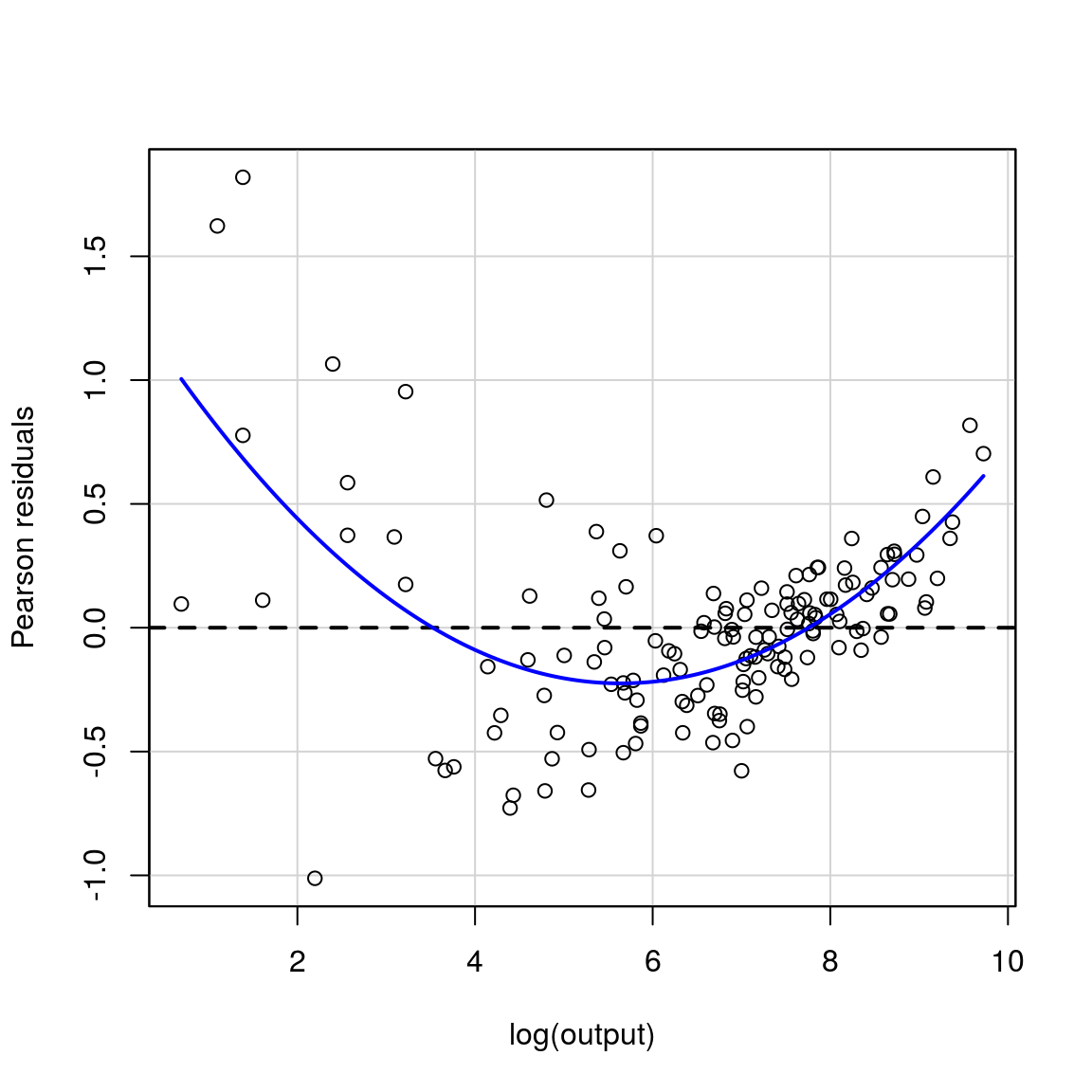
#> [1] "t stat is: 16.0195576357841"Importance of plotting residuals
The car package again helps us. car comes with a function residualPlot which will plot residuals against fitted values (by default), or against a specified variable, in our case log(output)
# residual plot comes from car package
residualPlot(model2, variable = "log(output)")