Application: Forward Exchange Rates as Optimal Predictors

Load the hayashir package

library(hayashir)

And other libraries we need for this chapter

library(dplyr) # data manipulation
#> 
#> Attaching package: 'dplyr'
#> The following objects are masked from 'package:stats':
#> 
#>     filter, lag
#> The following objects are masked from 'package:base':
#> 
#>     intersect, setdiff, setequal, union
library(ggplot2) # plotting
library(forecast) # time series plotting - Acf
library(sandwich) # HAC standard errors
library(lmtest)
#> Loading required package: zoo
#> 
#> Attaching package: 'zoo'
#> The following objects are masked from 'package:base':
#> 
#>     as.Date, as.Date.numeric
#> 
#> Attaching package: 'lmtest'
#> The following object is masked from 'package:hayashir':
#> 
#>     moneydemand
library(car)
#> Loading required package: carData
#> 
#> Attaching package: 'car'
#> The following object is masked from 'package:dplyr':
#> 
#>     recode

The Data

Let’s get a quick look at our data by looking at the first 10 rows:

head(yen, 10)
#> # A tibble: 10 x 4
#>    date       spot_rate forward_30 spot_30
#>    <date>         <dbl>      <dbl>   <dbl>
#>  1 1975-01-03      301.       301.    297.
#>  2 1975-01-10      301.       301.    295.
#>  3 1975-01-17      301.       300.    293.
#>  4 1975-01-24      296.       296.    286.
#>  5 1975-01-31      298.       298.    287.
#>  6 1975-02-07      296.       296.    286.
#>  7 1975-02-14      293.       293.    288.
#>  8 1975-02-21      291.       292.    288.
#>  9 1975-02-28      286.       286.    291.
#> 10 1975-03-07      286.       285.    292.

Figure 6.1: Forecast Error: Yen/Dollar


ggplot(data = yen, aes(x = date, y = spot_30 - forward_30))+
    geom_line() +
    geom_hline(yintercept = 0, linetype="dashed", color = "red") +
    theme_bw()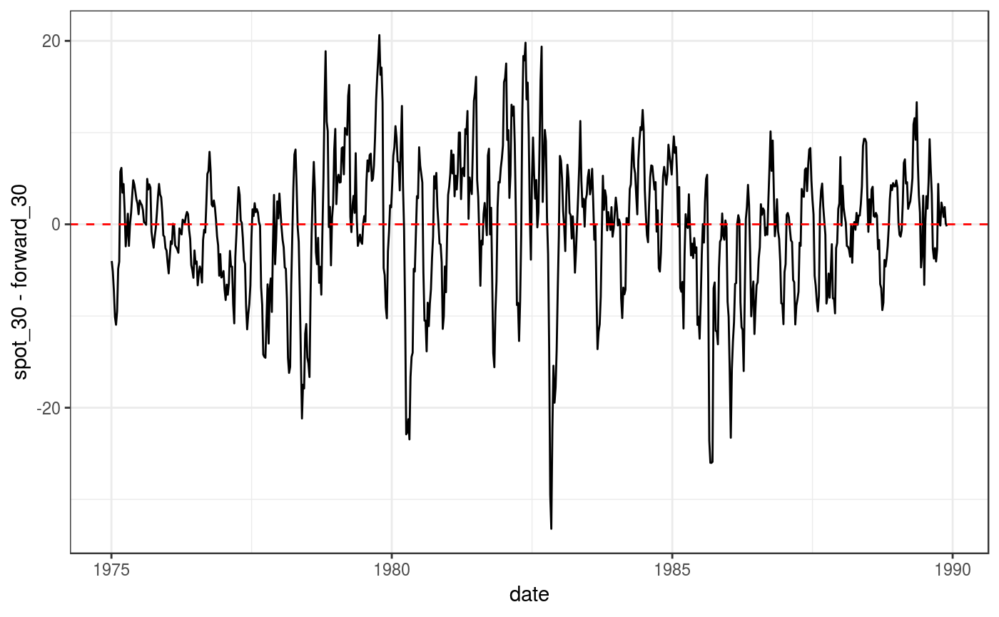

Figure 6.2: Correlogram of \(s30 - f\), Yen/Dollar

The Acf function from the forecast package will do what we need here:

Acf(yen$spot_30 - yen$forward_30, lag.max = 40)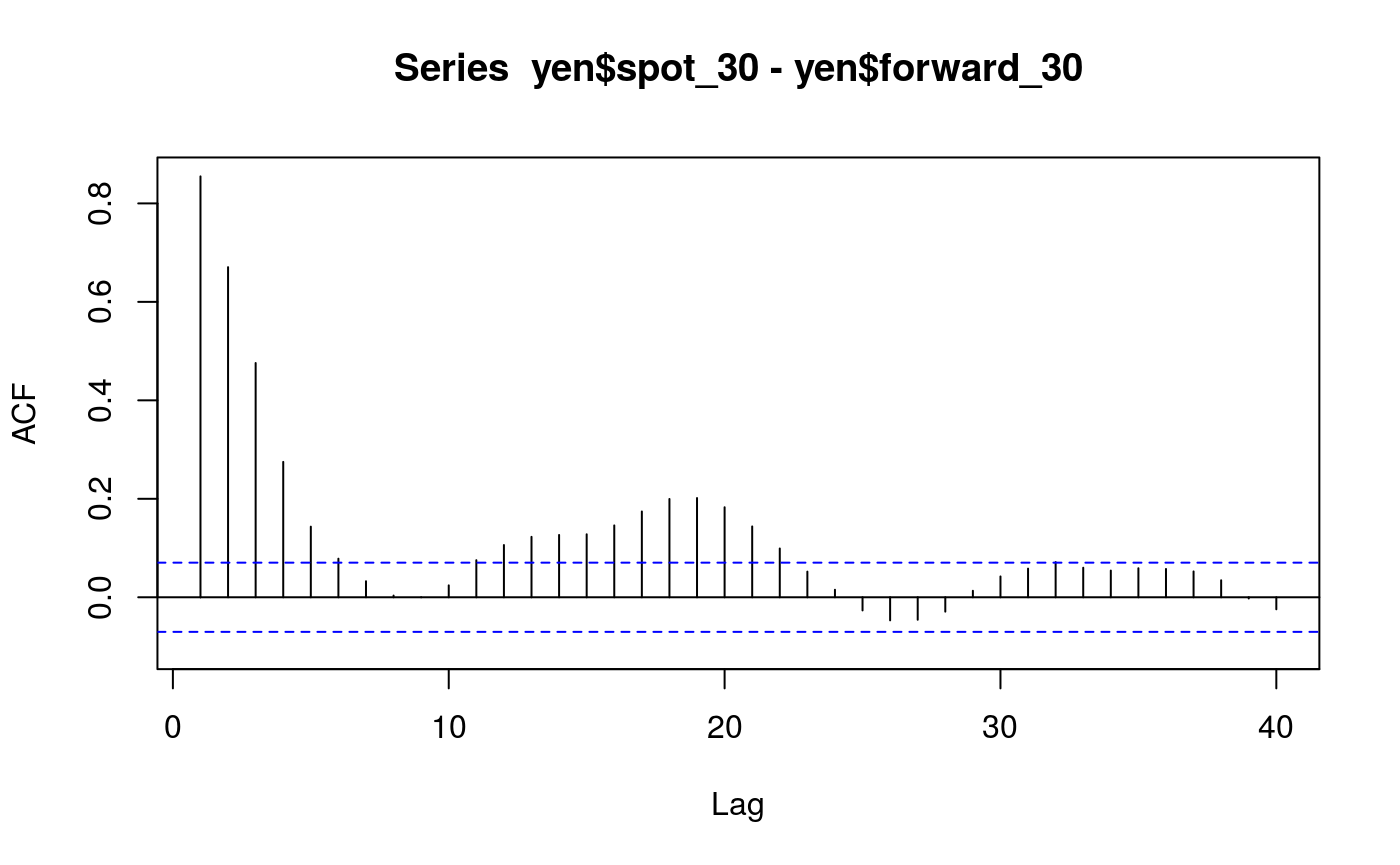

Figure 6.3: Yen/Dollar Spot Rate, Jan 1975 - Dec 1989

ggplot(data = yen, aes(x = date, y = spot_rate))+
    geom_line() +
    scale_x_date(date_breaks = "3 years", date_labels =  "%m/%y") +
    theme_bw()

Figure 6.4: Plot of \(s30\) against \(f\), Yen/Dollar

ggplot(data = yen, aes(x = log(forward_30), y = log(spot_30)))+
    geom_point() +
    theme_bw()

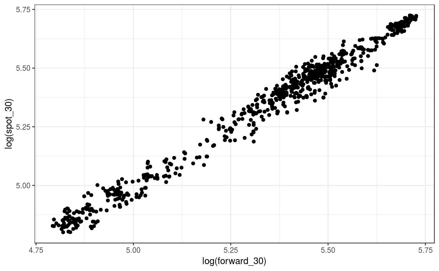
Table 6.2: Regression Tests for Market Efficiency

For the Yen/Dollar:

mkt_eff <- lm (I(spot_30 - spot_rate) ~ I(forward_30 - spot_rate), data = yen)

summary(mkt_eff)
#> 
#> Call:
#> lm(formula = I(spot_30 - spot_rate) ~ I(forward_30 - spot_rate), 
#>     data = yen)
#> 
#> Residuals:
#>     Min      1Q  Median      3Q     Max 
#> -33.105  -3.554   1.084   4.508  18.876 
#> 
#> Coefficients:
#>                           Estimate Std. Error t value Pr(>|t|)    
#> (Intercept)                -1.9700     0.3507  -5.618 2.70e-08 ***
#> I(forward_30 - spot_rate)  -1.6783     0.3720  -4.512 7.42e-06 ***
#> ---
#> Signif. codes:  0 '***' 0.001 '**' 0.01 '*' 0.05 '.' 0.1 ' ' 1
#> 
#> Residual standard error: 7.21 on 776 degrees of freedom
#> Multiple R-squared:  0.02556,    Adjusted R-squared:  0.02431 
#> F-statistic: 20.36 on 1 and 776 DF,  p-value: 7.424e-06

These results give standard errors under the assumption of heteroskedasticity. To correct for heteroskedasticity and autocorrelation we want HAC standard errors from the sandwich package. In particular standard errors with a maximum of 4 lags that are not pre-whitened. To get a summary of the regression we use the coeftest function from the lm package

coeftest(mkt_eff, vcov = vcovHAC(mkt_eff, lag = 4, prewhite = FALSE))
#> 
#> t test of coefficients:
#> 
#>                           Estimate Std. Error t value Pr(>|t|)   
#> (Intercept)               -1.96996    0.70083 -2.8109 0.005065 **
#> I(forward_30 - spot_rate) -1.67835    0.68199 -2.4610 0.014073 * 
#> ---
#> Signif. codes:  0 '***' 0.001 '**' 0.01 '*' 0.05 '.' 0.1 ' ' 1

To test that \(\beta_0 =0\) and \(\beta_1 = 1\) we use the linearHypothesis function from car

linearHypothesis(mkt_eff, c("(Intercept) = 0", "I(forward_30 - spot_rate) = 1"),
                 vcov = vcovHAC(mkt_eff, lag = 4, prewhite = FALSE))
#> Linear hypothesis test
#> 
#> Hypothesis:
#> (Intercept) = 0
#> I(forward_30 - spot_rate) = 1
#> 
#> Model 1: restricted model
#> Model 2: I(spot_30 - spot_rate) ~ I(forward_30 - spot_rate)
#> 
#> Note: Coefficient covariance matrix supplied.
#> 
#>   Res.Df Df      F    Pr(>F)    
#> 1    778                        
#> 2    776  2 8.1846 0.0003037 ***
#> ---
#> Signif. codes:  0 '***' 0.001 '**' 0.01 '*' 0.05 '.' 0.1 ' ' 1

Figure 6.5: Plot of \(s30-s\) against \(f - s\), Yen/Dollar

ggplot(data = yen, aes(x = forward_30 - spot_rate, y = spot_30 - spot_rate))+
    geom_point() +
    geom_smooth(method = "lm", se = FALSE, color = "red") +
    theme_bw()

Chapter 06: Serial Correlation

Lachlan Deer

2019-03-04