Chapter 02: Large Sample Theory

Load Libraries

library(hayashir)
library(ggplot2)
library(dplyr)
#> 
#> Attaching package: 'dplyr'
#> The following objects are masked from 'package:stats':
#> 
#>     filter, lag
#> The following objects are masked from 'package:base':
#> 
#>     intersect, setdiff, setequal, union
library(zoo)
#> 
#> Attaching package: 'zoo'
#> The following objects are masked from 'package:base':
#> 
#>     as.Date, as.Date.numeric

Inspecting the Data

head(mishkin)
#> # A tibble: 6 x 7
#>    year month inflation_1 inflation_3 tbill_1 tbill_3   cpi
#>   <dbl> <dbl>       <dbl>       <dbl>   <dbl>   <dbl> <dbl>
#> 1  1950     2       -3.55        1.13    1.10    1.13  23.5
#> 2  1950     3        5.25        4.00    1.13    1.14  23.6
#> 3  1950     4        1.69        4.49    1.12    1.14  23.6
#> 4  1950     5        5.06        7.82    1.15    1.18  23.7
#> 5  1950     6        6.72        9.43    1.16    1.17  23.8
#> 6  1950     7       11.7         9.98    1.15    1.17  24.1

Figure 2.3

First we construct a date variable and then calculate CPI inflation The library zoo contains the function as.yearmon() to construct dates containing only year and months.


mishkin2 <- mishkin %>%
                mutate(time_period = as.yearmon(paste(year, month, sep = "-")),
                       cpi_inflation = (cpi/lag(cpi) - 1) * 100 * 12
                       )

Now we plot the data:

ggplot(mishkin2) +
    geom_line(aes(time_period, tbill_1, linetype = "tbill_1")) +
    geom_line(aes(time_period, cpi_inflation, linetype = "cpi_inflation")) +
    xlab("Date") +
    ylab("percent") +
    theme_bw() + 
    theme(legend.position="bottom") +
    scale_linetype_manual(name = element_blank(), 
                          values = c(tbill_1 = "solid", cpi_inflation = "dotted"),
                          labels = c("inflation rate", "1 month T-bill rate")
                          )
#> Don't know how to automatically pick scale for object of type yearmon. Defaulting to continuous.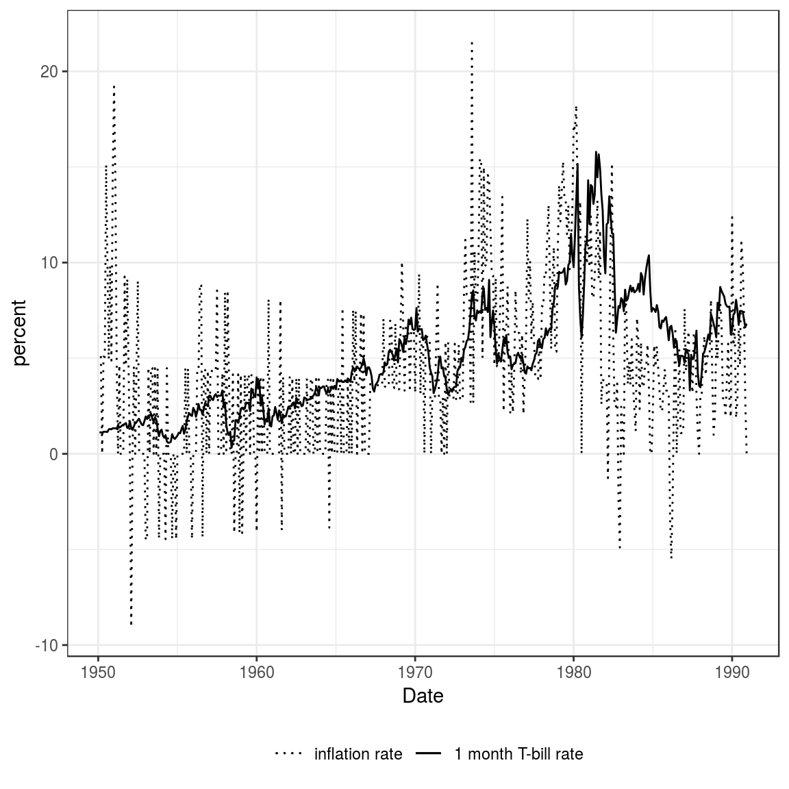

Figure 2.4

Compute real interest rate:

mishkin2 <- mishkin2 %>%
                mutate(real_rate = tbill_1 - cpi_inflation)

And now plot:

ggplot(mishkin2) +
    geom_line(aes(time_period, real_rate, linetype = "tbill_1")) +
    geom_hline(yintercept = 0, linetype = "dashed", color = "red") +
    xlab("Date") +
    ylab("percent") +
    theme_bw() + 
    theme(legend.position="none")
#> Don't know how to automatically pick scale for object of type yearmon. Defaulting to continuous.
#> Warning: Removed 1 rows containing missing values (geom_path).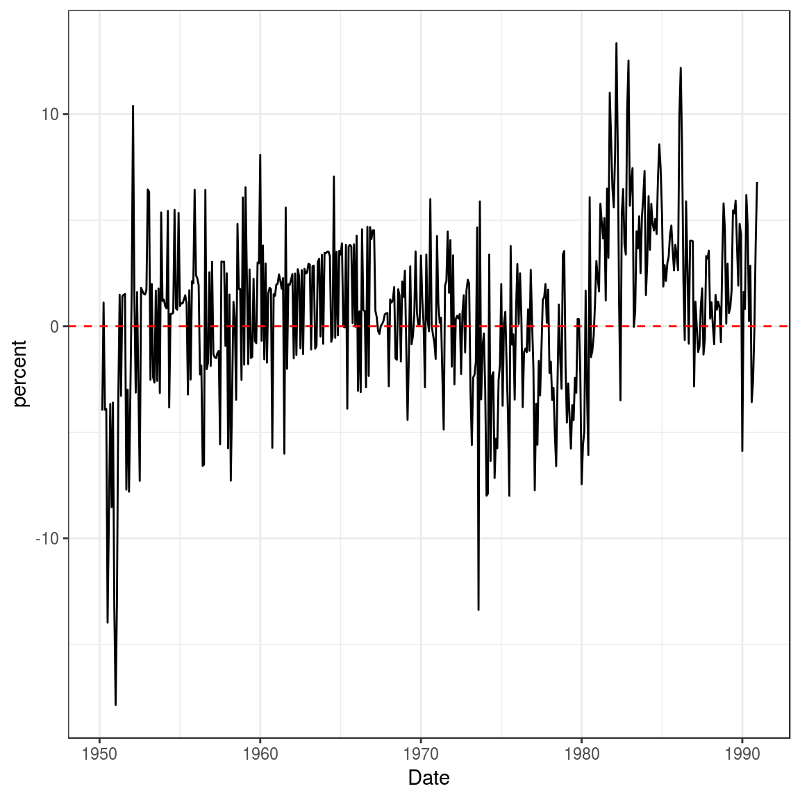

Table 2.1

First we subset the data. The relevant Date range is January 1953 to July 1971.

fama <- mishkin2 %>%
            filter(between(as.yearmon(time_period), 
                           as.yearmon("Jan 1953"), 
                           as.yearmon("Jul 1971")
                           )
                   )
#> Warning: between() called on numeric vector with S3 class

library(skimr)
skim(fama$real_rate)
#> Skim summary statistics
#> 
#> Variable type: numeric 
#>        variable missing complete   n mean   sd    p0   p25 median  p75
#>  fama$real_rate       0      223 223 0.89 2.77 -7.28 -0.99    1.1 2.77
#>  p100     hist
#>  8.08 ▁▁▃▆▇▆▂▁

Then the ACF

acf(fama$real_rate, lag.max = 12, plot = FALSE)
#> 
#> Autocorrelations of series 'fama$real_rate', by lag
#> 
#>      0      1      2      3      4      5      6      7      8      9 
#>  1.000 -0.105  0.173 -0.018 -0.007 -0.063 -0.025 -0.094  0.088  0.090 
#>     10     11     12 
#>  0.017  0.004  0.206

Then the Ljung Box Q tests (use the portes package for more flexibility)

library(portes)
#> Loading required package: parallel

LjungBox(fama$real_rate, lags = seq(1, 12))
#>  lags statistic df     p-value
#>     1  2.481488  1 0.115193236
#>     2  9.242763  2 0.009839194
#>     3  9.320394  3 0.025320868
#>     4  9.330291  4 0.053353656
#>     5 10.248907  5 0.068482075
#>     6 10.398756  6 0.108833047
#>     7 12.439184  7 0.087010028
#>     8 14.265193  8 0.075109784
#>     9 16.177062  9 0.063274884
#>    10 16.247091 10 0.092774254
#>    11 16.250588 11 0.132079904
#>    12 26.309947 12 0.009700248

Is the Nominal Interest Rate the Optimal Predictor?

model1 <- lm(cpi_inflation ~ tbill_1, data = fama)
summary(model1)
#> 
#> Call:
#> lm(formula = cpi_inflation ~ tbill_1, data = fama)
#> 
#> Residuals:
#>     Min      1Q  Median      3Q     Max 
#> -7.1795 -1.8660 -0.2112  1.8817  8.1608 
#> 
#> Coefficients:
#>             Estimate Std. Error t value Pr(>|t|)    
#> (Intercept)  -0.8699     0.4231  -2.056    0.041 *  
#> tbill_1       0.9930     0.1200   8.277  1.2e-14 ***
#> ---
#> Signif. codes:  0 '***' 0.001 '**' 0.01 '*' 0.05 '.' 0.1 ' ' 1
#> 
#> Residual standard error: 2.78 on 221 degrees of freedom
#> Multiple R-squared:  0.2366, Adjusted R-squared:  0.2332 
#> F-statistic: 68.51 on 1 and 221 DF,  p-value: 1.197e-14

How to get robust standard errors?

library(sandwich)
library(lmtest)
#> 
#> Attaching package: 'lmtest'
#> The following object is masked from 'package:hayashir':
#> 
#>     moneydemand

coeftest(model1, vcov = vcovHC(model1, "HC0")) # white's
#> 
#> t test of coefficients:
#> 
#>             Estimate Std. Error t value Pr(>|t|)    
#> (Intercept) -0.86987    0.42405 -2.0513  0.04141 *  
#> tbill_1      0.99301    0.10948  9.0702  < 2e-16 ***
#> ---
#> Signif. codes:  0 '***' 0.001 '**' 0.01 '*' 0.05 '.' 0.1 ' ' 1

library(car)
#> Loading required package: carData
#> 
#> Attaching package: 'car'
#> The following object is masked from 'package:dplyr':
#> 
#>     recode

linearHypothesis(model1, "tbill_1 = 1", white.adjust = "hc0")
#> Linear hypothesis test
#> 
#> Hypothesis:
#> tbill_1 = 1
#> 
#> Model 1: restricted model
#> Model 2: cpi_inflation ~ tbill_1
#> 
#> Note: Coefficient covariance matrix supplied.
#> 
#>   Res.Df Df      F Pr(>F)
#> 1    222                 
#> 2    221  1 0.0041 0.9492

Lachlan Deer

2019-03-04